Lab 8: Geoprocessing Services and Web Tools

Introduction

The goals of this lab were to develop a geoprocessing (GP) service using ModelBuilder in ArcMap and publishing the model as a service to a local server, then using that service to create a web app using ESRI's Web AppBuilder. The scenario for these initiatives included developing a web app that will allow end-users to find optimal locations for establishing a manufacturing industry. The criteria for candidacy includes: proximity to a river(s) and railroads, allows the user to enter a minimum population for a city, and select an area of interest. The GP service creates a buffer polygon layer of optimal locations.

Methods

To start this lab railroads, rivers, and Wisconsin cities layers were added to a blank ArcMap document. A new geodatabase and layer were created to store data and provide a blank feature layer to use for the area of interest selection in the model. A New>Toolbox was made in the project folder and New>Model opened up a blank model window (figures 1 and 2).

Figure 1: Create new toolbox.

Figure 2: Create new model.

The model was built by adding all of the geoprocessing tasks that were necessary to generate results for optimal locations. Various parameters were set to ensure the end-user meets all of the inputs required by the tool. Figure 3 shows the layout of the various tools, inputs, and outputs of the model.

Figure 3: Geoprocessing model.

Once the model was made, all parameters were established, and the inputs were configured, the geoprocessing environments were set to overwrite and save output files to the project geodatabase (figures 4 and 5).

Figure 4: Configuring geoprocessing options.

Figure 5: Set output and scratch workspace.

Next, the model was executed and requested that the end-user input a point of interest on the map (figures 6, 7, and 8).

Figure 6: Model running.

Figure 7: Select area of interest.

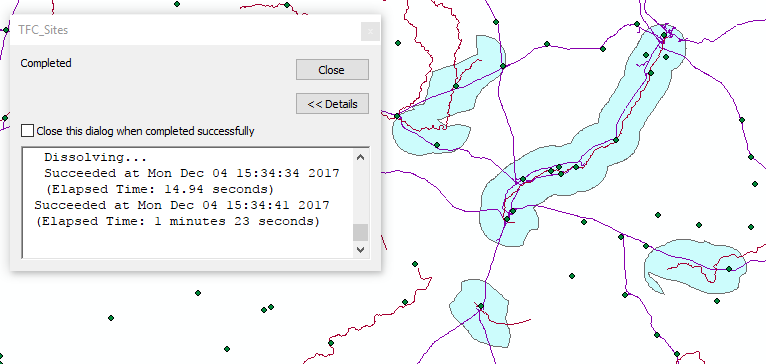
Figure 8: Completed running model. 

The blue areas in figure 8 show optimal areas for establishing a manufacturing industry based on the blue point selected in figure 7. Since the model worked, it was published as a service to a local server (figure 9).

Figure 9: Publish model as geoprocessing service.

The GP service was published to the local class server, which would be accessed later in the assignment to create a web app with this service (figure 10).

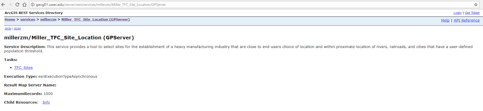
Figure 10: REST service located on class server.

Another service ModelBuilder provides is the ability to export any model to a Python script (figure 11). See resulting code in results section.

Figure 11: Export model to Python script.

Once the GP service was published to the class server, the service was published to the developer edition of Web AppBuilder using the development server. To do this, a new 2-D map was made and given a title in the Web AppBuilder. Then the GP service data was selected for the Choose Web Map function of the application (figure 12).

Figure 12: Select web map containing necessary data layers for the service.

Then the GP widget was configured to bring in the GP service created earlier (figure 13).

Figure 13: Enter the URL of the server that hosts the GP service. 

The service was validated and used to then configure the tool tips for each tool parameters. The application was then tested and published as a web service in the development server (figures 14 and 15).

Figure 14: Running GP task from web app.

Figure 15: Results of GP task test.

Results

Figure 16: Finished Web App.

The resulting service has the same functionality as in ArcMap or the in the editing process of Web AppBuilder, but looks clean and professional as well as has tool tips for input values when running GP task.

Having worked with ModelBuilder before, adding tools, setting inputs, and establishing parameters were all comfortable practices for me. I did not know, however, that finished models/tools created in ModelBuilder could be converted to Python scripts. This could be extremely useful for someone attempting to develop this app using scripting. I also thought that publishing the GP model as a service from ArcMap was useful.

Overall, the program works smoothly and effectively while still being relatively easy to develop and use. 

Python Script

# -*- coding: utf-8 -*-

# ---------------------------------------------------------------------------

# TCF_SitesScript.py

# Created on: 2017-12-04 15:37:41.00000

#   (generated by ArcGIS/ModelBuilder)

# Usage: TCF_SitesScript <Input_DistanceToRivers> <Input_DistanceToRails> <Input_PopulationValue> <Input_Location_of_Interest> <Input_DistanceOfInterest> <Factory_Optimal_Location> 

# Description: 

# ---------------------------------------------------------------------------

# Import arcpy module

import arcpy

# Script arguments

Input_DistanceToRivers = arcpy.GetParameterAsText(0)

if Input_DistanceToRivers == '#' or not Input_DistanceToRivers:

    Input_DistanceToRivers = "5 Kilometers" # provide a default value if unspecified

Input_DistanceToRails = arcpy.GetParameterAsText(1)

if Input_DistanceToRails == '#' or not Input_DistanceToRails:

    Input_DistanceToRails = "5 Kilometers" # provide a default value if unspecified

Input_PopulationValue = arcpy.GetParameterAsText(2)

if Input_PopulationValue == '#' or not Input_PopulationValue:

    Input_PopulationValue = "4000" # provide a default value if unspecified

Input_Location_of_Interest = arcpy.GetParameterAsText(3)

if Input_Location_of_Interest == '#' or not Input_Location_of_Interest:

    Input_Location_of_Interest = "in_memory\\{C84ECC84-6AF1-46B9-B156-A2A9C9704F4B}" # provide a default value if unspecified

Input_DistanceOfInterest = arcpy.GetParameterAsText(4)

if Input_DistanceOfInterest == '#' or not Input_DistanceOfInterest:

    Input_DistanceOfInterest = "50 Kilometers" # provide a default value if unspecified

Factory_Optimal_Location = arcpy.GetParameterAsText(5)

if Factory_Optimal_Location == '#' or not Factory_Optimal_Location:

    Factory_Optimal_Location = "Z:\\MILLERZM\\Lab8\\Lab8.gdb\\Rivers_Clip_Buffer_Intersect2" # provide a default value if unspecified

# Local variables:

Rivers = "Rivers"

Point_Buffer = "Z:\\MILLERZM\\Lab8\\Lab8.gdb\\Buffer"

Rivers_Clip = "Z:\\MILLERZM\\Lab8\\Lab8.gdb\\Rivers_Clip"

River_Buffer = "Z:\\MILLERZM\\Lab8\\Lab8.gdb\\Rivers_Clip_Buffer"

Railroads = "Railroads"

Railroad_Clip = "Z:\\MILLERZM\\Lab8\\Lab8.gdb\\Railroads_Clip"

Rail_Buffer = "Z:\\MILLERZM\\Lab8\\Lab8.gdb\\Railroads_Clip_Buffer"

River_Rail_Int = "Z:\\MILLERZM\\Lab8\\Lab8.gdb\\Rivers_Clip_Buffer_Intersect"

Wisconsin_Cities = "Wisconsin_Cities"

Wisconsin_Cities_Select = "Z:\\MILLERZM\\Lab8\\Lab8.gdb\\Wisconsin_Cities_Select"

Required_Cities_Clip = "Z:\\MILLERZM\\Lab8\\Lab8.gdb\\Wisconsin_Cities_Select_Clip"

Wisconsin_Cities_Select_Clip1 = "Z:\\MILLERZM\\Lab8\\Lab8.gdb\\Wisconsin_Cities_Select_Clip1"

All_Criteria = "Z:\\MILLERZM\\Lab8\\Lab8.gdb\\Rivers_Clip_Buffer_Intersect1"

# Process: Buffer1

arcpy.Buffer_analysis(Input_Location_of_Interest, Point_Buffer, Input_DistanceOfInterest, "FULL", "ROUND", "NONE", "", "PLANAR")

# Process: Clip1

arcpy.Clip_analysis(Rivers, Point_Buffer, Rivers_Clip, "")

# Process: Buffer2

arcpy.Buffer_analysis(Rivers_Clip, River_Buffer, Input_DistanceToRivers, "FULL", "ROUND", "NONE", "", "PLANAR")

# Process: Clip2

arcpy.Clip_analysis(Railroads, Point_Buffer, Railroad_Clip, "")

# Process: Buffer3

arcpy.Buffer_analysis(Railroad_Clip, Rail_Buffer, Input_DistanceToRails, "FULL", "ROUND", "NONE", "", "PLANAR")

# Process: Intersect

arcpy.Intersect_analysis("Z:\\MILLERZM\\Lab8\\Lab8.gdb\\Rivers_Clip_Buffer #;Z:\\MILLERZM\\Lab8\\Lab8.gdb\\Railroads_Clip_Buffer #", River_Rail_Int, "ALL", "", "INPUT")

# Process: Select

arcpy.Select_analysis(Wisconsin_Cities, Wisconsin_Cities_Select, "POP2007 >= 4000")

# Process: Clip3

arcpy.Clip_analysis(Wisconsin_Cities_Select, Point_Buffer, Required_Cities_Clip, "")

# Process: Select2

arcpy.Select_analysis(Required_Cities_Clip, Wisconsin_Cities_Select_Clip1, "")

# Process: Spatial Join

arcpy.SpatialJoin_analysis(River_Rail_Int, Wisconsin_Cities_Select_Clip1, All_Criteria, "JOIN_ONE_TO_ONE", "KEEP_ALL", "FID_Rivers_Clip_Buffer \"FID_Rivers_Clip_Buffer\" true true false 0 Long 0 0 ,First,#,Z:\\MILLERZM\\Lab8\\Lab8.gdb\\Rivers_Clip_Buffer_Intersect,FID_Rivers_Clip_Buffer,-1,-1;IHABBSRF_I \"IHABBSRF_I\" true true false 8 Double 0 0 ,First,#,Z:\\MILLERZM\\Lab8\\Lab8.gdb\\Rivers_Clip_Buffer_Intersect,IHABBSRF_I,-1,-1;RR \"RR\" true true false 11 Text 0 0 ,First,#,Z:\\MILLERZM\\Lab8\\Lab8.gdb\\Rivers_Clip_Buffer_Intersect,RR,-1,-1;HUC \"HUC\" true true false 4 Long 0 0 ,First,#,Z:\\MILLERZM\\Lab8\\Lab8.gdb\\Rivers_Clip_Buffer_Intersect,HUC,-1,-1;TYPE \"TYPE\" true true false 1 Text 0 0 ,First,#,Z:\\MILLERZM\\Lab8\\Lab8.gdb\\Rivers_Clip_Buffer_Intersect,TYPE,-1,-1;PNAME \"PNAME\" true true false 30 Text 0 0 ,First,#,Z:\\MILLERZM\\Lab8\\Lab8.gdb\\Rivers_Clip_Buffer_Intersect,PNAME,-1,-1;OWNAME \"OWNAME\" true true false 30 Text 0 0 ,First,#,Z:\\MILLERZM\\Lab8\\Lab8.gdb\\Rivers_Clip_Buffer_Intersect,OWNAME,-1,-1;PNMCD \"PNMCD\" true true false 11 Text 0 0 ,First,#,Z:\\MILLERZM\\Lab8\\Lab8.gdb\\Rivers_Clip_Buffer_Intersect,PNMCD,-1,-1;OWNMCD \"OWNMCD\" true true false 11 Text 0 0 ,First,#,Z:\\MILLERZM\\Lab8\\Lab8.gdb\\Rivers_Clip_Buffer_Intersect,OWNMCD,-1,-1;DSRR \"DSRR\" true true false 8 Double 0 0 ,First,#,Z:\\MILLERZM\\Lab8\\Lab8.gdb\\Rivers_Clip_Buffer_Intersect,DSRR,-1,-1;DSHUC \"DSHUC\" true true false 4 Long 0 0 ,First,#,Z:\\MILLERZM\\Lab8\\Lab8.gdb\\Rivers_Clip_Buffer_Intersect,DSHUC,-1,-1;USDIR \"USDIR\" true true false 1 Text 0 0 ,First,#,Z:\\MILLERZM\\Lab8\\Lab8.gdb\\Rivers_Clip_Buffer_Intersect,USDIR,-1,-1;LEV \"LEV\" true true false 4 Long 0 0 ,First,#,Z:\\MILLERZM\\Lab8\\Lab8.gdb\\Rivers_Clip_Buffer_Intersect,LEV,-1,-1;J \"J\" true true false 4 Long 0 0 ,First,#,Z:\\MILLERZM\\Lab8\\Lab8.gdb\\Rivers_Clip_Buffer_Intersect,J,-1,-1;TERMID \"TERMID\" true true false 4 Long 0 0 ,First,#,Z:\\MILLERZM\\Lab8\\Lab8.gdb\\Rivers_Clip_Buffer_Intersect,TERMID,-1,-1;TRMBLV \"TRMBLV\" true true false 4 Long 0 0 ,First,#,Z:\\MILLERZM\\Lab8\\Lab8.gdb\\Rivers_Clip_Buffer_Intersect,TRMBLV,-1,-1;K \"K\" true true false 4 Long 0 0 ,First,#,Z:\\MILLERZM\\Lab8\\Lab8.gdb\\Rivers_Clip_Buffer_Intersect,K,-1,-1;Miles \"Miles\" true true false 8 Double 0 0 ,First,#,Z:\\MILLERZM\\Lab8\\Lab8.gdb\\Rivers_Clip_Buffer_Intersect,Miles,-1,-1;Shape_Length \"Shape_Length\" true true true 8 Double 0 0 ,First,#,Z:\\MILLERZM\\Lab8\\Lab8.gdb\\Rivers_Clip_Buffer_Intersect,Shape_Length,-1,-1;Shape_length_1 \"Shape_length_1\" true true false 0 Double 0 0 ,First,#,Z:\\MILLERZM\\Lab8\\Lab8.gdb\\Rivers_Clip_Buffer_Intersect,Shape_length_1,-1,-1;BUFF_DIST \"BUFF_DIST\" true true false 0 Double 0 0 ,First,#,Z:\\MILLERZM\\Lab8\\Lab8.gdb\\Rivers_Clip_Buffer_Intersect,BUFF_DIST,-1,-1;ORIG_FID \"ORIG_FID\" true true false 0 Long 0 0 ,First,#,Z:\\MILLERZM\\Lab8\\Lab8.gdb\\Rivers_Clip_Buffer_Intersect,ORIG_FID,-1,-1;FID_Railroads_Clip_Buffer \"FID_Railroads_Clip_Buffer\" true true false 0 Long 0 0 ,First,#,Z:\\MILLERZM\\Lab8\\Lab8.gdb\\Rivers_Clip_Buffer_Intersect,FID_Railroads_Clip_Buffer,-1,-1;ObjectID_1 \"ObjectID_1\" true true false 4 Long 0 0 ,First,#,Z:\\MILLERZM\\Lab8\\Lab8.gdb\\Rivers_Clip_Buffer_Intersect,ObjectID_1,-1,-1;ID \"ID\" true true false 4 Long 0 0 ,First,#,Z:\\MILLERZM\\Lab8\\Lab8.gdb\\Rivers_Clip_Buffer_Intersect,ID,-1,-1;RAILROAD \"RAILROAD\" true true false 31 Text 0 0 ,First,#,Z:\\MILLERZM\\Lab8\\Lab8.gdb\\Rivers_Clip_Buffer_Intersect,RAILROAD,-1,-1;RROWNER \"RROWNER\" true true false 4 Text 0 0 ,First,#,Z:\\MILLERZM\\Lab8\\Lab8.gdb\\Rivers_Clip_Buffer_Intersect,RROWNER,-1,-1;TR \"TR\" true true false 4 Text 0 0 ,First,#,Z:\\MILLERZM\\Lab8\\Lab8.gdb\\Rivers_Clip_Buffer_Intersect,TR,-1,-1;PASSENGER \"PASSENGER\" true true false 4 Text 0 0 ,First,#,Z:\\MILLERZM\\Lab8\\Lab8.gdb\\Rivers_Clip_Buffer_Intersect,PASSENGER,-1,-1;MILITARY \"MILITARY\" true true false 1 Text 0 0 ,First,#,Z:\\MILLERZM\\Lab8\\Lab8.gdb\\Rivers_Clip_Buffer_Intersect,MILITARY,-1,-1;FRA_REG \"FRA_REG\" true true false 2 Text 0 0 ,First,#,Z:\\MILLERZM\\Lab8\\Lab8.gdb\\Rivers_Clip_Buffer_Intersect,FRA_REG,-1,-1;CLASS \"CLASS\" true true false 1 Text 0 0 ,First,#,Z:\\MILLERZM\\Lab8\\Lab8.gdb\\Rivers_Clip_Buffer_Intersect,CLASS,-1,-1;MILES_1 \"MILES_1\" true true false 8 Double 0 0 ,First,#,Z:\\MILLERZM\\Lab8\\Lab8.gdb\\Rivers_Clip_Buffer_Intersect,MILES_1,-1,-1;Shape_Length_12 \"Shape_Length_12\" true true true 8 Double 0 0 ,First,#,Z:\\MILLERZM\\Lab8\\Lab8.gdb\\Rivers_Clip_Buffer_Intersect,Shape_Length_12,-1,-1;Shape_length_12_13 \"Shape_length_12_13\" true true false 0 Double 0 0 ,First,#,Z:\\MILLERZM\\Lab8\\Lab8.gdb\\Rivers_Clip_Buffer_Intersect,Shape_length_12_13,-1,-1;BUFF_DIST_1 \"BUFF_DIST_1\" true true false 0 Double 0 0 ,First,#,Z:\\MILLERZM\\Lab8\\Lab8.gdb\\Rivers_Clip_Buffer_Intersect,BUFF_DIST_1,-1,-1;ORIG_FID_1 \"ORIG_FID_1\" true true false 0 Long 0 0 ,First,#,Z:\\MILLERZM\\Lab8\\Lab8.gdb\\Rivers_Clip_Buffer_Intersect,ORIG_FID_1,-1,-1;Shape_length_12_13_14 \"Shape_length_12_13_14\" true true false 0 Double 0 0 ,First,#,Z:\\MILLERZM\\Lab8\\Lab8.gdb\\Rivers_Clip_Buffer_Intersect,Shape_length,-1,-1;Shape_area \"Shape_area\" true true false 0 Double 0 0 ,First,#,Z:\\MILLERZM\\Lab8\\Lab8.gdb\\Rivers_Clip_Buffer_Intersect,Shape_area,-1,-1;ObjectID \"ObjectID\" true true false 4 Long 0 0 ,First,#,Z:\\MILLERZM\\Lab8\\Lab8.gdb\\Wisconsin_Cities_Select_Clip1,ObjectID,-1,-1;FEATURE \"FEATURE\" true true false 21 Text 0 0 ,First,#,Z:\\MILLERZM\\Lab8\\Lab8.gdb\\Wisconsin_Cities_Select_Clip1,FEATURE,-1,-1;NAME \"NAME\" true true false 48 Text 0 0 ,First,#,Z:\\MILLERZM\\Lab8\\Lab8.gdb\\Wisconsin_Cities_Select_Clip1,NAME,-1,-1;ST_ABBREV \"ST_ABBREV\" true true false 2 Text 0 0 ,First,#,Z:\\MILLERZM\\Lab8\\Lab8.gdb\\Wisconsin_Cities_Select_Clip1,ST_ABBREV,-1,-1;FIPS \"FIPS\" true true false 5 Text 0 0 ,First,#,Z:\\MILLERZM\\Lab8\\Lab8.gdb\\Wisconsin_Cities_Select_Clip1,FIPS,-1,-1;PLACE_FIPS \"PLACE_FIPS\" true true false 5 Text 0 0 ,First,#,Z:\\MILLERZM\\Lab8\\Lab8.gdb\\Wisconsin_Cities_Select_Clip1,PLACE_FIPS,-1,-1;POP_2000 \"POP_2000\" true true false 4 Long 0 0 ,First,#,Z:\\MILLERZM\\Lab8\\Lab8.gdb\\Wisconsin_Cities_Select_Clip1,POP_2000,-1,-1;POP2007 \"POP2007\" true true false 4 Long 0 0 ,First,#,Z:\\MILLERZM\\Lab8\\Lab8.gdb\\Wisconsin_Cities_Select_Clip1,POP2007,-1,-1;STATUS \"STATUS\" true true false 30 Text 0 0 ,First,#,Z:\\MILLERZM\\Lab8\\Lab8.gdb\\Wisconsin_Cities_Select_Clip1,STATUS,-1,-1", "INTERSECT", "", "")

# Process: Dissolve

arcpy.Dissolve_management(All_Criteria, Factory_Optimal_Location, "", "", "MULTI_PART", "DISSOLVE_LINES")

Sources

Zach Miller
Dr. Cyril Wilson
ESRI

Lab 7: Volunteered Geographic Information (VGI)

Introduction

The purpose of this lab was to develop mobile responsive apps that are comprised of Volunteered Geographic Information (VGI). VGI is geographic data that is contributed by end-users of an application- in this case, to document the condition of fire hydrants, sidewalks, and green spaces. Using an attachment function, the end-user can upload pictures of the feature/s they're uploading.

Methods

Part 1:

In order to allow end-users to upload information to a map, they must have a map with features to access and update. In the first part of this lab, a map containing three feature classes was created in ArcMap, published as a service, and enabled feature access. This was done by first creating new feature classes in a geodatabase (figures 1 and 2).

Figure 1: Establishing domains and subtypes for feature classes.

In figure 1, rules for the feature classes to be added to the geodatabase are established, the coded values (options for an end user to select) are created, and data types for feature classes are set. Once this was done, the new feature classes were added to the geodatabase (figure 2), using the parameters set in the previous step.

Figure 2: Creating a new feature class.

Next, an attachment option was created (figure 3) for the sidewalk and fire hydrant classes. This setting would allow end-users to add attachments to their uploaded features in the resulting webpage app.

Figure 3: Create attachment capabilities.

Now, the end-user can add features and attachments to those features to the map (figures 4 and 5).

Figure 4: Add fire hydrant point feature to map. 

Figure 5: Attach picture to user-plotted point.

Then, the map was published to a local server to be accessed as a service in the following code.

Part 2:

Essentially the same code for the latter two parts that make up this lab was used, with a few modifications to add a toggle button to open/close the attribute upload window for users to contribute VGI. The first HTML code used (figure 6) establishes the webpage content and references the stylesheets and other code used to give functionality to the webpage.

Figure 6: HTML document.

The next section of code was a JavaScript document (figures 7 and 8) which gives the webpage its functional elements such as accessing the necessary Dojo libraries, enabling end-users to add features to the map, and ensuring topology integrity of line and polygon features.

Figure 7: JavaScript document (1/2).

Figure 8: JavaScript document (2/2).

Next, a CSS document was created to establish sizes and aesthetic features of the webpage (figure 9).

Figure 9: CSS document.

Once all of these documents were created, the html code was launched. This resulted in a webpage where users can access feature layers to upload and attach images to (see Results section).

Part 3:

For the last part of this lab, the original HTML, JavaScript, and CSS documents were copied and edited an another JavaScript document was created to enable the toggle feature added to this section. The HTML code received a few changes which include: an Apple status bar in the apple mobile app configuration of the webpage, reference to the toggle JavaScript document, and a window for the toggle function (figure 10).

Figure 10: HTML document.

Next, the original JavaScript code was copied and used again for this section (figures 11 and 12).

Figure 11: JavaScript document (1/2). 

Figure 12: JavaScript document (2/2).

Then, the original CSS document was modified to include a template picker pane styling, a toggle on/off button, and the feature layers window styling (figures 13 and 14).

Figure 13: CSS document (1/2).

Figure 14: CSS document (2/2).

Lastly, the toggle functionality and parameters were established using a seprate JavaScript document (figure 15).

Figure 15: Toggle JavaScript document.

Results

Figure 16: First VGI webpage without toggle feature.

Figure 17: Second VGI webpage with toggle feature.

Figure 18: Adding a feature to the map.

Results

Using a VGI app or webpage could certainly have many useful applications. From the scenario used in this lab (updating fire hydrant, sidewalk, and/or green space information), to reporting crimes, there are quite literally infinite possibilities with VGI interfaces. 

Although its use is relatively easy, the underlying code for this VGI was quite tricky to write. With multiple servers used and various languages/documents to keep track of, writing this script took some time. I felt as though the toggle feature didn't add much functionality to the application other than providing more screen space for mobile users.

Overall, this is a very useful technology that can provide access to everyday citizens of a place to improve their community, business, or project. With a little bit of time, access to ArcMap, and knowledge of coding, anyone has the ability to create and utilize a VGI interface.

Sources

Zach Miller
Dr. Cyril Wilson
ESRI

Lab 6: Mobile Responsive Apps

Introduction

Expanding on the previous lab, the goal of this assignment was to develop a webpage that is responsive to mobile applications. The benefit of having a mobile responsive webpage is that it allows the end-user to access the webpage's content from multiple platforms- keeping the client satisfied with your product. Using pieces of code from ArcGIS API for JavaScript and DOM*, the results of this lab were: a places, addresses, congressional districts, senators' information, and higher education search application; and a query application that returns graphical and text information for Wisconsin counties. 

Methods

Part 1 - Section I

To start these objectives, an HTML document was created. This document references the necessary ArcGIS JavaScript stylesheets, viewport for iOS and Android mobile responsiveness, and some CSS code for map and search widget styling (figure 1).

Figure 1: Search app HTML document.

Next, a JavaScript document was created which references the Map, Search, FeatureLayer, and InfoTemplate dojo libraries. Within the functions shown in figures 2 and 3, various parameters are set to ensure the objects display and function properly.

Figure 2: Search app JavaScript document.

Figure 3: Search app JavaScript document continued.

With the two documents working together, the code produced a search application site for end-users to search congressional districts, senators, and geocode addresses (see results). 

Part 1 - Section II

For the next section of this activity, the code generated in section one was modified to support a universities search service instead of senators. To achieve this, a shapefile containing location information of universities in the U.S. was published to the local UW-Eau Claire geography server (see Lab 2). Then, that service URL was referenced in the JavaScript document (figure 4).

Figure 4: Search app with universities JavaScript document.

The beginning part of the .js code was the same as in section 1 (see figure 2). As with the JavaScript code, a copy of the HTML document from section 1 was made and edited to reference the new JavaScript document (figure 5).

Figure 5: Search app with universities HTML document. 

The application was then launched in a web browser and provided a search option for universities instead of senators (see results section).

Part 2

For the next part of this lab, a query app which allows end-users to visualize how the populations of each county in Wisconsin compares to the most populous county in the state. To begin this task, an HTML document was created (figure 6) and referenced the appropriate styling sheets, the associated JavaScript document, and the associated CSS document.

Figure 6: HTML document.

Then, the JavaScript document (figure 7) was used to establish connections to the appropriate dojo libraries, all of the API and predeveloped application functions, and dynamic graphics to display the data.

Figure 7: JavaScript document.

Lastly, a CSS document was made (figure 8) to establish the aesthetic properties of the dynamic gauge infographic and webpage containers. 

Figure 8: CSS document.

The HTML code was launched in a web browser and displayed a well-designed query service (see results section).

Results

Figure 9: Resulting web application.

As seen in figure 9, the resulting application is visually and functionally pleasing. The most populous county in Wisconsin is Milwaukee county of course, so when the end-user hovers over Dane county (figure 9), they can see that the county has 51% of the population that Milwaukee county has.

Creating this app was a bit tedious and required a lot of details for such a dynamic data info graphic, but the result turned out superb. Using the dynamic info graphics from ESRI in a web application can really make it appear more sophisticated and provide some exciting data visualization for the end-user.

Sources

Zach Miller
Dr. Cyril Wilson
ArcGIS API for JavaScript 

Lab 5: ArcGIS API for JavaScript 1

Introduction

The purpose of this lab was to connect concepts of JavaScript, HTML, and CSS learned in previous labs and access ESRI’s ArcGIS JavaScript Application Programming Interface (API). The API allows the programmer to use and customize various web GIS components from templates. In this case specifically, these templates utilize ESRI frameworks- meaning the functioning components (ie. basemaps, symbols, and even pre-packaged web services) in the resulting web pages are designed by ESRI.

Methods

Part 1:
To start this lab, a new HTML document was created. This HTML code set up a basic GIS service webpage, giving the site a title ("Create a Map"), URL, and an ESRI basemap as the content (figure 1).

Figure 1: "Create a Map" HTML document.

Next, a new JavaScript document was created (figure 2). This script established access to various web app components from ESRI JavaScript API, used components from the Dojo library, and set the extent for the basemap. This script, and it's components, works by referencing the file name in the original HTML code (see "Miller_p1.js" in figure 1).

Figure 2: "Create a Map" JavaScript document.

Part 2 - Section I:
In the next part of this lab, an HTML and JavaScript document were set up in the same way as in part 1. This time, however, a pre-packaged web service was accessed within the code using a variety of functions within the JavaScript document. In figure 3, the HTML code for this section is shown.

Figure 3: "Custom Info Window" HTML document.

Looking at figure 3, a <script> within the HTML code was added; the dojoConfig variable. This script accesses a module stored within the project folder that loads when the web page is accessed. Again, the JavaScript file (figure 4) was referenced in this code which contains the dynamic elements of the page, access to the pre-packaged web service, and size of components on the web page.

Figure 4: "Custom Info Window" JavaScript document.

Most of the functionality of the web page is contained within the code shown in figure 4. As with the previous JavaScript document, various components of the dojo library are listed to be accessed later in the script. The different variables (var) and functions (function) are set-up. The pre-packaged web service was accessed with the "new FeatureLayer" variable in line 41, for example.

Part 2 - Section II
Using a pre-packaged web service to practice accessing them in HTML is just that- good practice. For the next section of this part of the lab, a new web service was produced, published, and then accessed within the JavaScript document (figure #). To start, a shapefile containing school locations in Eau Claire county was brought into ArcMap and symbolized. The shapefile used didn't contain the addresses of the schools, however, a separate data table within the project folder did. The tables of the two layers were joined by school name (figure 5).

Figure 5: Table join in ArcMap.

It was important to validate the join before joining to ensure cardinality. Once the tables were joined, the shapefile data was exported as a new shapefile (figure 6).

Figure 6: Export data to new shapefile.

Then, copies of attribute fields from the table join were removed to leave the fields that would display in a pop-up on the resulting web page: Name of school (NAME), elevation of school in meters (ELEV_METER), and address of school (ADDRESS). Next, the map was published to the class server as a service in a similar way to the second lab of this course.

Using the JavaScript document created in the previous section as a template, a copy was made and edited to fit the requirements for this webpage. In figure 7, the new JavaScript document is shown.

Figure 7: Eau Claire Schools JavaScript document.

Looking at figure 7, some changes are noticeable. For instance, the coordinates for the center of the map extent have changed as well as the zoom. The feature layer variable contains the server URL where the Eau Claire school service is stored. Furthermore, a scale bar was added (lines 36-39), the pop-up window content and aliases were configured (line 44), the infoWindow size was changed to accommodate the data displayed in the pop-up window (line 54), and the getTextContext graphic function was removed. In the HTML document, the appropriate JavaScript document was referenced (see figure 8).

Figure 8: Eau Claire Schools HTML document.

Part 3:

For the last part of this lab, a routing application was developed. To begin, a new HTML document was created (figure 9); setting up the script in a similar way to previous HTML documents in this lab. For this web page the ESRI .css stylesheet "claro" was used to style the web page.

Figure 9: Simple Routing HTML document.

Looking at figure 9, the appropriate JavaScript document (figures 10 and 11) was referenced and some text was added to display instructions under the map window of the web page.

Figure 10: Simple Routing JavaScript requirements section. 

Figure 11: Simple Routing JavaScript continued.

As shown in figure 11, the server where the routing web service is stored was referenced in the routeTask variable, the point and line symbols were configured, and an error message was set up among other web page functions.

Results

Part 1

Figure 12: Create a Map webpage.

Part 2 - Section I

Figure 13: Custom Info Window webpage.

Part 2 - Section II

Figure 14: Eau Claire Schools webpage.

Part 3

Figure 15: Simple Routing webpage.

Results

While this lab was certainly difficult, I thought it did a good job of exposing me to different modules, libraries, APIs, and the overall capabilities of using JavaScript, HTML, and CSS to develop web pages. Most of the problems I ran into while completing this lab were due to minor spelling or symbol errors, however, this is the nature of working with programming languages. Lastly, I found this exercise useful in expanding my knowledge of various code components that make up functions within a web page. For example, calling the various dojo functions within the require statement in the JavaScript codes is essential to defining each function's parameters later in the script.

Sources

EC_Schools feature class was obtained from MapCruzin.com at: http://www.mapcruzin.com/geographic-names-shapefiles/#School

EC_Schools_Address was assembled by GEOG 455 class, fall 2013. Widget_infowindow files were provided by Esri at:
https://developers.arcgis.com/javascript/jssamples.html

A reference to explain cardinality was used:
https://en.wikipedia.org/wiki/Cardinality_(data_modeling)

Source code provided by:
Dr. Cyril Wilson, GEOG 455: Web GIS, Fall 2017